How to use Naive Bayes Theorem in Machine Learning

January 2025
M	T	W	T	F	S	S
	1	2	3	4	5
6	7	8	9	10	11	12
13	14	15	16	17	18	19
20	21	22	23	24	25	26
27	28	29	30	31

Suppose you are a product manager, you want to classify customer reviews in positive and negative classes. Or As a loan manager, you want to identify which loan applicants are safe or risky? As a healthcare analyst, you want to predict which patients can suffer from diabetes disease. All the examples have the same kind of problem to classify reviews, loan applicants, and patients.

Naive Bayes is the most straightforward and fast classification algorithm, which is suitable for a large chunk of data. Naive Bayes classifier is successfully used in various applications such as spam filtering, text classification, sentiment analysis, and recommender systems. It uses Bayes theorem of probability for prediction of unknown class.

In this tutorial, you are going to learn about all of the following:

Classification Workflow
What is Naive Bayes classifier?
How Naive Bayes classifier works?
Classifier building in Scikit-learn
Zero Probability Problem
It’s advantages and disadvantages

To easily run all the example code in this tutorial yourself, you can create a DataLab workbook for free that has Python pre-installed and contains all code samples. For more practice on scikit-learn, check out our Supervised Learning with Scikit-learn course!

Become a ML Scientist

Master Python skills to become a machine learning scientist

Start Learning for Free

Classification Workflow

Whenever you perform classification, the first step is to understand the problem and identify potential features and label. Features are those characteristics or attributes which affect the results of the label. For example, in the case of a loan distribution, bank managers identify the customer’s occupation, income, age, location, previous loan history, transaction history, and credit score. These characteristics are known as features that help the model classify customers.

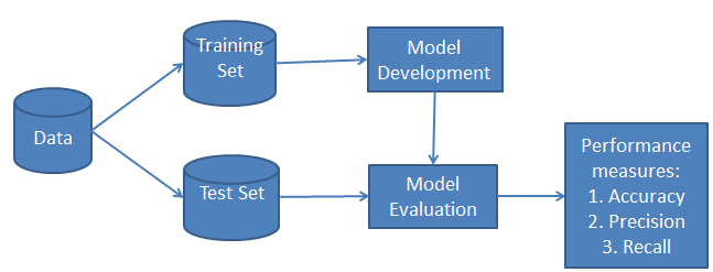
The classification has two phases, a learning phase and the evaluation phase. In the learning phase, the classifier trains its model on a given dataset, and in the evaluation phase, it tests the classifier’s performance. Performance is evaluated on the basis of various parameters such as accuracy, error, precision, and recall.

What is Naive Bayes Classifier?

Naive Bayes is a statistical classification technique based on Bayes Theorem. It is one of the simplest supervised learning algorithms. Naive Bayes classifier is the fast, accurate and reliable algorithm. Naive Bayes classifiers have high accuracy and speed on large datasets.

Naive Bayes classifier assumes that the effect of a particular feature in a class is independent of other features. For example, a loan applicant is desirable or not depending on his/her income, previous loan and transaction history, age, and location. Even if these features are interdependent, these features are still considered independently. This assumption simplifies computation, and that’s why it is considered as naive. This assumption is called class conditional independence.

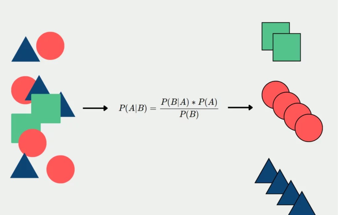
P(h): the probability of hypothesis h being true (regardless of the data). This is known as the prior probability of h.
P(D): the probability of the data (regardless of the hypothesis). This is known as the prior probability.
P(h|D): the probability of hypothesis h given the data D. This is known as posterior probability.
P(D|h): the probability of data d given that the hypothesis h was true. This is known as posterior probability.

How Naive Bayes Classifier Works?

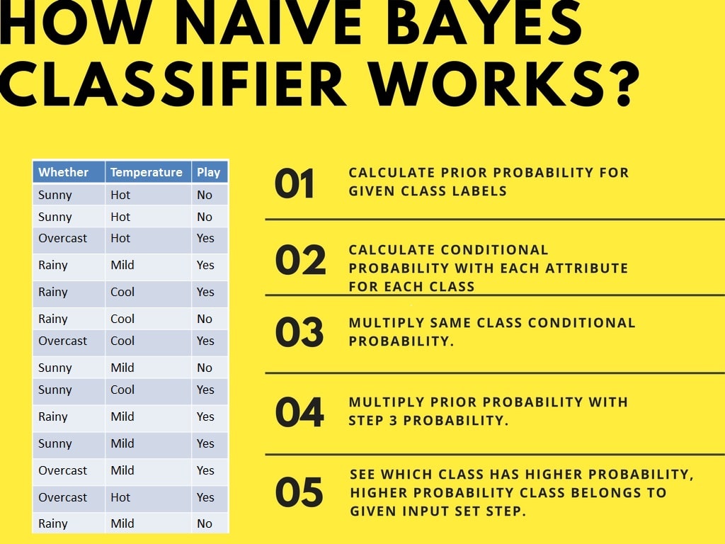
Let’s understand the working of Naive Bayes through an example. Given an example of weather conditions and playing sports. You need to calculate the probability of playing sports. Now, you need to classify whether players will play or not, based on the weather condition.

First Approach (In case of a single feature)

Naive Bayes classifier calculates the probability of an event in the following steps:

Step 1: Calculate the prior probability for given class labels
Step 2: Find Likelihood probability with each attribute for each class
Step 3: Put these value in Bayes Formula and calculate posterior probability.
Step 4: See which class has a higher probability, given the input belongs to the higher probability class.

For simplifying prior and posterior probability calculation, you can use the two tables frequency and likelihood tables. Both of these tables will help you to calculate the prior and posterior probability. The Frequency table contains the occurrence of labels for all features. There are two likelihood tables. Likelihood Table 1 is showing prior probabilities of labels and Likelihood Table 2 is showing the posterior probability.

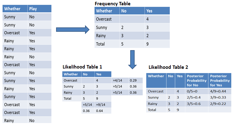
Now suppose you want to calculate the probability of playing when the weather is overcast.

Probability of playing:

P(Yes | Overcast) = P(Overcast | Yes) P(Yes) / P (Overcast) …………………(1)

Calculate Prior Probabilities:

P(Overcast) = 4/14 = 0.29

P(Yes)= 9/14 = 0.64

Calculate Posterior Probabilities:

P(Overcast |Yes) = 4/9 = 0.44

Put Prior and Posterior probabilities in equation (1)

P (Yes | Overcast) = 0.44 * 0.64 / 0.29 = 0.98(Higher)

Similarly, you can calculate the probability of not playing:

Probability of not playing:

P(No | Overcast) = P(Overcast | No) P(No) / P (Overcast) …………………(2)

Calculate Prior Probabilities:

P(Overcast) = 4/14 = 0.29

P(No)= 5/14 = 0.36

Calculate Posterior Probabilities:

P(Overcast |No) = 0/9 = 0

Put Prior and Posterior probabilities in equation (2)

P (No | Overcast) = 0 * 0.36 / 0.29 = 0

The probability of a ‘Yes’ class is higher. So you can determine here if the weather is overcast than players will play the sport.

Second Approach (In case of multiple features)

Now suppose you want to calculate the probability of playing when the weather is overcast, and the temperature is mild.

Probability of playing:

P(Play= Yes | Weather=Overcast, Temp=Mild) = P(Weather=Overcast, Temp=Mild | Play= Yes)P(Play=Yes) ……….(1)

P(Weather=Overcast, Temp=Mild | Play= Yes)= P(Overcast |Yes) P(Mild |Yes) ………..(2)

Calculate Prior Probabilities: P(Yes)= 9/14 = 0.64
Calculate Posterior Probabilities: P(Overcast |Yes) = 4/9 = 0.44 P(Mild |Yes) = 4/9 = 0.44
Put Posterior probabilities in equation (2) P(Weather=Overcast, Temp=Mild | Play= Yes) = 0.44 * 0.44 = 0.1936(Higher)
Put Prior and Posterior probabilities in equation (1) P(Play= Yes | Weather=Overcast, Temp=Mild) = 0.1936*0.64 = 0.124

Similarly, you can calculate the probability of not playing:

Probability of not playing:

P(Play= No | Weather=Overcast, Temp=Mild) = P(Weather=Overcast, Temp=Mild | Play= No)P(Play=No) ……….(3)

P(Weather=Overcast, Temp=Mild | Play= No)= P(Weather=Overcast |Play=No) P(Temp=Mild | Play=No) ………..(4)

Calculate Prior Probabilities: P(No)= 5/14 = 0.36
Calculate Posterior Probabilities: P(Weather=Overcast |Play=No) = 0/9 = 0 P(Temp=Mild | Play=No)=2/5=0.4
Put posterior probabilities in equation (4) P(Weather=Overcast, Temp=Mild | Play= No) = 0 * 0.4= 0
Put prior and posterior probabilities in equation (3) P(Play= No | Weather=Overcast, Temp=Mild) = 0*0.36=0

The probability of a ‘Yes’ class is higher. So you can say here that if the weather is overcast than players will play the sport.

Classifier Building in Scikit-learn

Naive Bayes Classifier with Synthetic Dataset

In the first example, we will generate synthetic data using scikit-learn and train and evaluate the Gaussian Naive Bayes algorithm.

Generating the Dataset

Scikit-learn provides us with a machine learning ecosystem so that you can generate the dataset and evaluate various machine learning algorithms.

In our case, we are creating a dataset with six features, three classes, and 800 samples using the make_classification function.

from sklearn.datasets import make_classification

X, y = make_classification(
    n_features=6,
    n_classes=3,
    n_samples=800,
    n_informative=2,
    random_state=1,
    n_clusters_per_class=1,
)

from sklearn.datasets import make_classification

X, y = make_classification(

n_features=6,

n_classes=3,

n_samples=800,

n_informative=2,

random_state=1,

n_clusters_per_class=1,

)

We will use matplotlib.pyplot’s scatter function to visualize the dataset.

import matplotlib.pyplot as plt

plt.scatter(X[:, 0], X[:, 1], c=y, marker="*");

import matplotlib.pyplot as plt

plt.scatter(X[:, 0], X[:, 1], c=y, marker="*");

As we can observe, there are three types of target labels, and we will be training a multiclass classification model.

Train Test Split

Before we start the training process, we need to split the dataset into training and testing for model evaluation.

from sklearn.model_selection import train_test_split

X_train, X_test, y_train, y_test = train_test_split(
    X, y, test_size=0.33, random_state=125
)

from sklearn.model_selection import train_test_split

X_train, X_test, y_train, y_test = train_test_split(

X, y, test_size=0.33, random_state=125

)

Model Building and Training

Build a generic Gaussian Naive Bayes and train it on a training dataset. After that, feed a random test sample to the model to get a predicted value.

from sklearn.naive_bayes import GaussianNB

# Build a Gaussian Classifier
model = GaussianNB()

# Model training
model.fit(X_train, y_train)

# Predict Output
predicted = model.predict([X_test[6]])

print("Actual Value:", y_test[6])
print("Predicted Value:", predicted[0])

from sklearn.naive_bayes import GaussianNB

# Build a Gaussian Classifier

model = GaussianNB()

# Model training

model.fit(X_train, y_train)

# Predict Output

predicted = model.predict([X_test[6]])

print("Actual Value:", y_test[6])

print("Predicted Value:", predicted[0])

Both actual and predicted values are the same.

Actual Value: 0
Predicted Value: 0

1 2	Actual Value: 0 Predicted Value: 0

Model Evaluation

We will not evolve the model on an unseen test dataset. First, we will predict the values for the test dataset and use them to calculate accuracy and F1 score.

from sklearn.metrics import (
    accuracy_score,
    confusion_matrix,
    ConfusionMatrixDisplay,
    f1_score,
)

y_pred = model.predict(X_test)
accuray = accuracy_score(y_pred, y_test)
f1 = f1_score(y_pred, y_test, average="weighted")

print("Accuracy:", accuray)
print("F1 Score:", f1)

from sklearn.metrics import (

accuracy_score,

confusion_matrix,

ConfusionMatrixDisplay,

f1_score,

)

y_pred = model.predict(X_test)

accuray = accuracy_score(y_pred, y_test)

f1 = f1_score(y_pred, y_test, average="weighted")

print("Accuracy:", accuray)

print("F1 Score:", f1)

Our model has performed fairly well with default hyperparameters.

Accuracy: 0.8484848484848485
F1 Score: 0.8491119695890328

1 2	Accuracy: 0.8484848484848485 F1 Score: 0.8491119695890328

To visualize the Confusion matrix, we will use confusion_matrix to calculate the true positives and true negatives and ConfusionMatrixDisplay to display the confusion matrix with the labels.

labels = [0,1,2]
cm = confusion_matrix(y_test, y_pred, labels=labels)
disp = ConfusionMatrixDisplay(confusion_matrix=cm, display_labels=labels)
disp.plot();

labels = [0,1,2]

cm = confusion_matrix(y_test, y_pred, labels=labels)

disp = ConfusionMatrixDisplay(confusion_matrix=cm, display_labels=labels)

disp.plot();

Our model has performed quite well, and we can improve model performance by scaling, preprocessing cross-validations, and hyperparameter optimization.

Naive Bayes Classifier with Loan Dataset

Let’s train the Naive Bayes Classifier on the real dataset. We will be repeating most of the tasks except for preprocessing and data exploration.

Data Loading

In this example, we will be loading Loan Data from DataLab using the pandas ‘read_csv function.




		
		
			
			

			
			import pandas as pd


df = pd.read_csv('loan_data.csv')
df.head()
			
				
					
				
					1
2
3
4
5
				
						import pandas as pd
 
 
df = pd.read_csv('loan_data.csv')
df.head()
					
				
			
		


Data Exploration

To understand more about the dataset we will use .info().



The dataset consists of 14 columns and 9578 rows.
Apart from “purpose”, columns are either floats or integers.
Our target column is “not.fully.paid”.



		
		
			
			

			
			df.info()
			
				
					
				
					1
				
						df.info()
					
				
			
		



		
		
			
			

			
			RangeIndex: 9578 entries, 0 to 9577
Data columns (total 14 columns):
#   Column             Non-Null Count  Dtype 
---  ------             --------------  ----- 
0   credit.policy      9578 non-null   int64 
1   purpose            9578 non-null   object
2   int.rate           9578 non-null   float64
3   installment        9578 non-null   float64
4   log.annual.inc     9578 non-null   float64
5   dti                9578 non-null   float64
6   fico               9578 non-null   int64 
7   days.with.cr.line  9578 non-null   float64
8   revol.bal          9578 non-null   int64 
9   revol.util         9578 non-null   float64
10  inq.last.6mths     9578 non-null   int64 
11  delinq.2yrs        9578 non-null   int64 
12  pub.rec            9578 non-null   int64 
13  not.fully.paid     9578 non-null   int64 
dtypes: float64(6), int64(7), object(1)
memory usage: 1.0+ MB
			
				
					
				
					1
2
3
4
5
6
7
8
9
10
11
12
13
14
15
16
17
18
19
20
				
						RangeIndex: 9578 entries, 0 to 9577
Data columns (total 14 columns):
#   Column             Non-Null Count  Dtype 
---  ------             --------------  ----- 
0   credit.policy      9578 non-null   int64 
1   purpose            9578 non-null   object
2   int.rate           9578 non-null   float64
3   installment        9578 non-null   float64
4   log.annual.inc     9578 non-null   float64
5   dti                9578 non-null   float64
6   fico               9578 non-null   int64 
7   days.with.cr.line  9578 non-null   float64
8   revol.bal          9578 non-null   int64 
9   revol.util         9578 non-null   float64
10  inq.last.6mths     9578 non-null   int64 
11  delinq.2yrs        9578 non-null   int64 
12  pub.rec            9578 non-null   int64 
13  not.fully.paid     9578 non-null   int64 
dtypes: float64(6), int64(7), object(1)
memory usage: 1.0+ MB
					
				
			
		


In this example, we will be developing a model to predict the customers who have not fully paid the loan. Let’s explore the purpose and target column by using seaborn’s countplot.


		
		
			
			

			
			import seaborn as sns
import matplotlib.pyplot as plt

sns.countplot(data=df,x='purpose',hue='not.fully.paid')
plt.xticks(rotation=45, ha='right');
			
				
					
				
					1
2
3
4
5
				
						import seaborn as sns
import matplotlib.pyplot as plt
 
sns.countplot(data=df,x='purpose',hue='not.fully.paid')
plt.xticks(rotation=45, ha='right');
					
				
			
		


Our dataset is an imbalance that will affect the performance of the model. You can check out Resample an Imbalanced Dataset tutorial to get hands-on experience in handling imbalanced datasets.
Data Processing

We will now convert the ‘purpose’ column from categorical to integer using pandas get_dummies function.




		
		
			
			

			
			pre_df = pd.get_dummies(df,columns=['purpose'],drop_first=True)
pre_df.head()
			
				
					
				
					1
2
				
						pre_df = pd.get_dummies(df,columns=['purpose'],drop_first=True)
pre_df.head()
					
				
			
		


After that, we will define feature (X) and target (y) variables, and split the dataset into training and testing sets.


		
		
			
			

			
			from sklearn.model_selection import train_test_split

X = pre_df.drop('not.fully.paid', axis=1)
y = pre_df['not.fully.paid']

X_train, X_test, y_train, y_test = train_test_split(
    X, y, test_size=0.33, random_state=125
)
			
				
					
				
					1
2
3
4
5
6
7
8
				
						from sklearn.model_selection import train_test_split
 
X = pre_df.drop('not.fully.paid', axis=1)
y = pre_df['not.fully.paid']
 
X_train, X_test, y_train, y_test = train_test_split(
    X, y, test_size=0.33, random_state=125
)
					
				
			
		


Model Building and Training
Model building and training is quite simple. We will be training a model on a training dataset using default hyperparameters.


		
		
			
			

			
			from sklearn.naive_bayes import GaussianNB

model = GaussianNB()

model.fit(X_train, y_train);
			
				
					
				
					1
2
3
4
5
				
						from sklearn.naive_bayes import GaussianNB
 
model = GaussianNB()
 
model.fit(X_train, y_train);
					
				
			
		


Model Evaluation
We will use accuracy and f1 score to determine model performance, and it looks like the Gaussian Naive Bayes algorithm has performed quite well.


		
		
			
			

			
			from sklearn.metrics import (
    accuracy_score,
    confusion_matrix,
    ConfusionMatrixDisplay,
    f1_score,
    classification_report,
)

y_pred = model.predict(X_test)

accuray = accuracy_score(y_pred, y_test)
f1 = f1_score(y_pred, y_test, average="weighted")

print("Accuracy:", accuray)
print("F1 Score:", f1)
			
				
					
				
					1
2
3
4
5
6
7
8
9
10
11
12
13
14
15
				
						from sklearn.metrics import (
    accuracy_score,
    confusion_matrix,
    ConfusionMatrixDisplay,
    f1_score,
    classification_report,
)
 
y_pred = model.predict(X_test)
 
accuray = accuracy_score(y_pred, y_test)
f1 = f1_score(y_pred, y_test, average="weighted")
 
print("Accuracy:", accuray)
print("F1 Score:", f1)
					
				
			
		



		
		
			
			

			
			Accuracy: 0.8206263840556786
F1 Score: 0.8686606980013266
			
				
					
				
					1
2
				
						Accuracy: 0.8206263840556786
F1 Score: 0.8686606980013266

Due to the imbalanced nature of the data, we can see that the confusion matrix tells a different story. On a minority target: not fully paid`, we have more mislabeled.

labels = ["Fully Paid", "Not fully Paid"]
cm = confusion_matrix(y_test, y_pred)
disp = ConfusionMatrixDisplay(confusion_matrix=cm, display_labels=labels)
disp.plot();

labels = ["Fully Paid", "Not fully Paid"]

cm = confusion_matrix(y_test, y_pred)

disp = ConfusionMatrixDisplay(confusion_matrix=cm, display_labels=labels)

disp.plot();

If you are facing issues during training or model evaluation, you can check out Naive Bayes Classification Tutorial using Scikit-learn DataLab workbook. It comes with a dataset, source code, and outputs.

Zero Probability Problem

Suppose there is no tuple for a risky loan in the dataset; in this scenario, the posterior probability will be zero, and the model is unable to make a prediction. This problem is known as Zero Probability because the occurrence of the particular class is zero.

The solution for such an issue is the Laplacian correction or Laplace Transformation. Laplacian correction is one of the smoothing techniques. Here, you can assume that the dataset is large enough that adding one row of each class will not make a difference in the estimated probability. This will overcome the issue of probability values to zero.

For Example: Suppose that for the class loan risky, there are 1000 training tuples in the database. In this database, the income column has 0 tuples for low income, 990 tuples for medium income, and 10 tuples for high income. The probabilities of these events, without the Laplacian correction, are 0, 0.990 (from 990/1000), and 0.010 (from 10/1000)

Now, apply Laplacian correction on the given dataset. Let’s add 1 more tuple for each income-value pair. The probabilities of these events:

Advantages

It is not only a simple approach but also a fast and accurate method for prediction.
Naive Bayes has a very low computation cost.
It can efficiently work on a large dataset.
It performs well in case of discrete response variable compared to the continuous variable.
It can be used with multiple class prediction problems.
It also performs well in the case of text analytics problems.
When the assumption of independence holds, a Naive Bayes classifier performs better compared to other models like logistic regression.

Disadvantages

The assumption of independent features. In practice, it is almost impossible that model will get a set of predictors which are entirely independent.
If there is no training tuple of a particular class, this causes zero posterior probability. In this case, the model is unable to make predictions. This problem is known as Zero Probability/Frequency Problem.

Conclusion

Congratulations, you have made it to the end of this tutorial!

In this tutorial, you learned about Naïve Bayes algorithm, its working, Naive Bayes assumption, issues, implementation, advantages, and disadvantages. Along the road, you have also learned model building and evaluation in scikit-learn for binary and multinomial classes.

Naive Bayes is the most straightforward and potent algorithm. In spite of the significant advances in machine learning in the last couple of years, it has proved its worth. It has been successfully deployed in many applications, from text analytics to recommendation engines.